This project implements a real-time audio spectrum analyser using a PIC18F4550 8-bit microcontroller. The spectrum frequency analysis is performed by a highly optimised 16-bit Fast Fourier Transformation (FFT) routine coded entirely in C. The output from the FFT is displayed using a 128×64 graphical LCD to allow a real-time view of an audio signal.

YouTube Demonstration Video

Hardware

In order to perform a FFT calculation on an audio signal it is necessary to prepare the audio so the PIC18F4550 can sample the signal. The PIC18F4550 provides several analogue to digital converters (ADCs) which can be used to measure a voltage from 0V to 5V with 10-bit accuracy (0-1023). A typical audio line-out signal is an analogue wave with a peak-to-peak intensity of 2V centred around 0V (i.e. it is an AC signal ranging from +1 to -1V) as shown by the following oscilloscope trace (from pin W2 of the demo board):

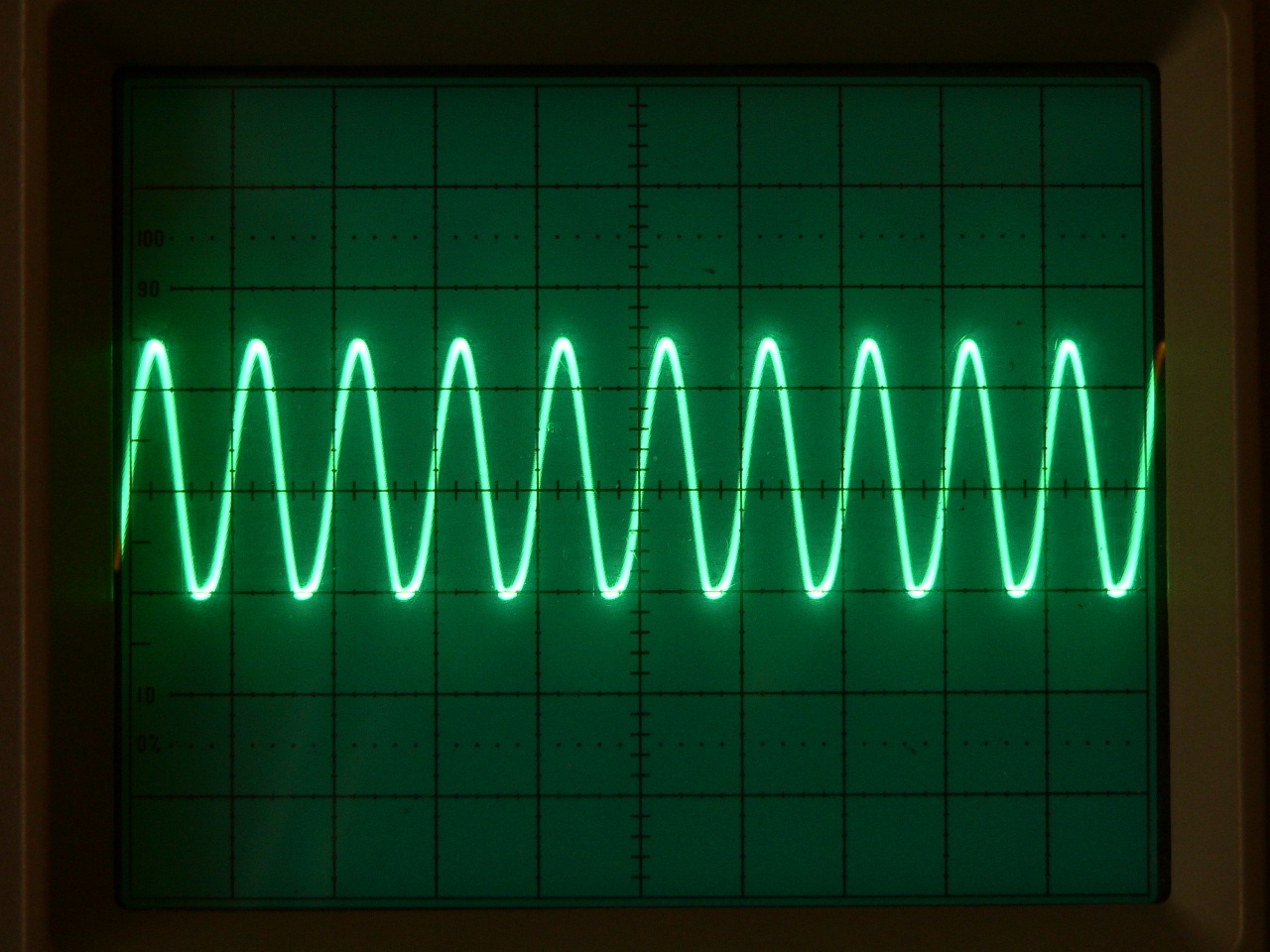
The picture shows a full-volume 5000Hz sine wave generated by a PC. If we were to feed this signal directly to the PIC we would only have a very small range of input voltage (0-0.5V) and also we would only be able to sample the top-half of the signal which would make the FFT incorrect.

In order to correctly sample the signal we have to do two things. Firstly we need to amplify the signal to ensure we can use as much of the 0-5V range as possible. Secondly we have to move the signal’s ground (of 0 volts) to a ‘virtual ground’ of 2.5Vs. This will allow the PIC to sample both the positive and the negative sides of the input signal. To do this the demonstration board uses a simple amplifier IC (the LM386-1). Since the IC is powered from a 0V and 5V power supply it has the handy side-effect of also moving the signal into the middle of our required power range. The LM386-1 was used because it is cheap and simple, however you could use a rail-to-rail opamp to achieve the same thing with a few more external components.

The following oscilloscope trace shows the output signal from the LM386-1 (for the signal shown above), the scope voltage range is set to 5 volts (from pin W3 of the demo board):

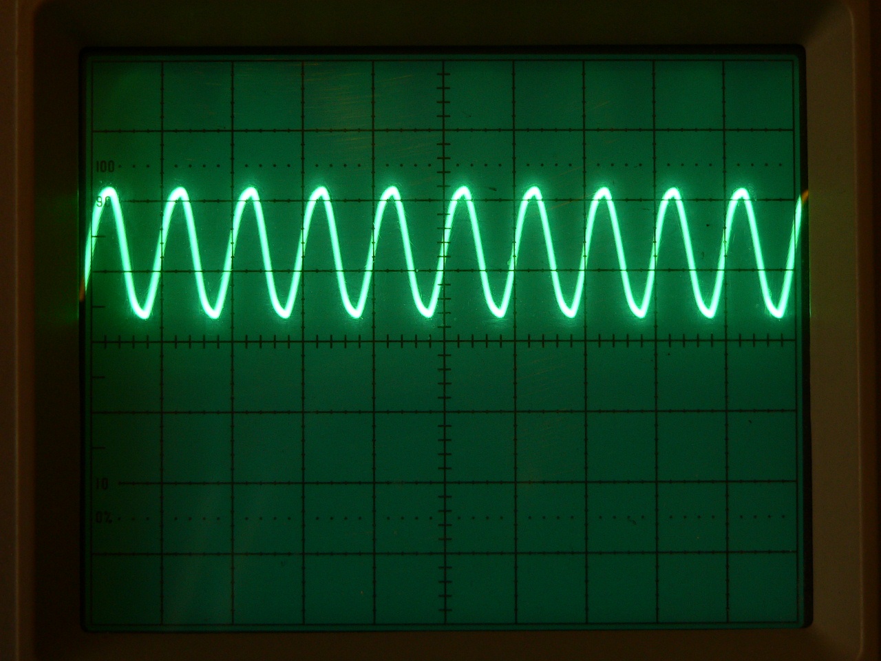
The hardware mixes the stereo line-in using two 10K resistors which act as a simple mixer. The signal is then passed to the LM386-1 via a 10K potentiometer which allows the signal strength to be adjusted. Next the LM386-1 amplifier output is passed through a simple RC Filter which rolls off the signal at about 10Khz. The resulting signal is then fed into an ADC pin on the PIC18F4550. The 10Khz filter acts as an ‘anti-aliasing’ filter for the FFT which cannot correctly detect signals with a frequency of greater than 10KHz. An RC filter is a very simple type of filter (and very ineffective) but it was chosen since it is easy to build and only requires 2 passive components. Typically a professional spectrum analyser would implement the anti-alias filter at 80% of the Nyquist frequency for the FFT (see below), but since we are so speed-limited with the PIC this is not possible to do in the design.

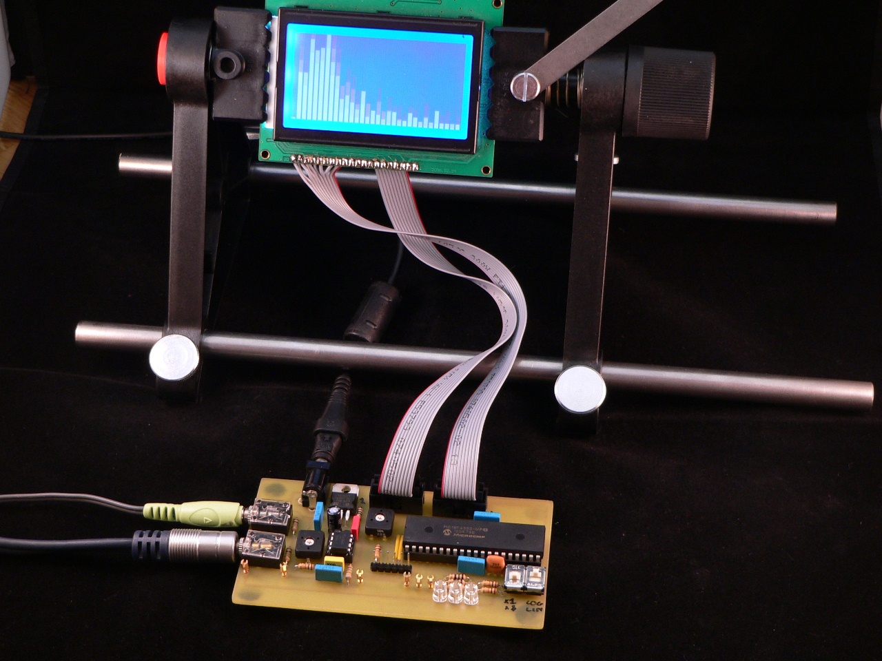
The demo board also controls a standard 128×64 dot-matrix LCD as well as 3 LEDs (for testing sound-to-light conversion). In addition there are 2 switches to allow the user to control the LCD’s output depending on what is being measured and how it is to be displayed. The second phono socket allows you to pass-through the input signal to another audio device such as headphones or speakers.

Here is the circuit schematic for the demonstration board:

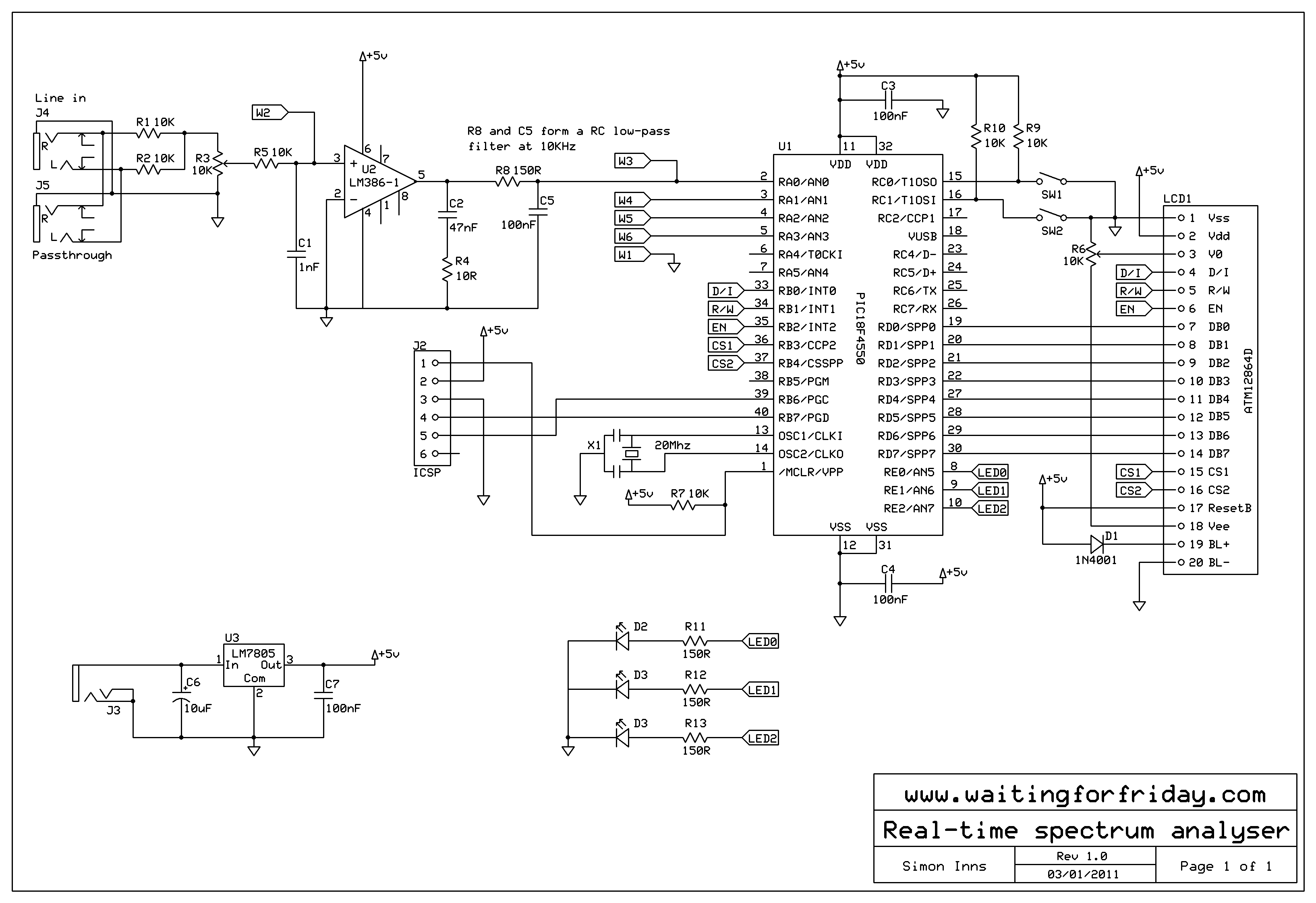
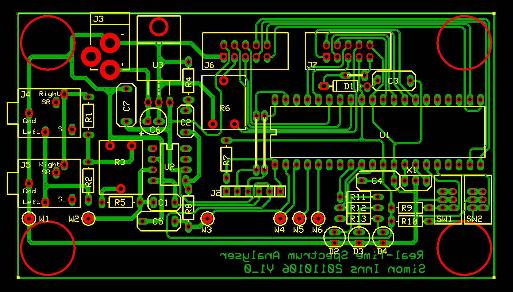
The circuit board design is a single-layer PCB using only through-hole components to make it as easy as possible to duplicate. I used a PIC18F4550 for the extra I/O pins however it can be directly replaced with the smaller PIC18F2550 which is code-compatible. The circuit is also simple enough to be built easily on a breadboard if you wish to experiment with the design. Here is a picture of the PCB artwork which is included in the downloads section below:

Firmware

The firmware is completely written in C and can be downloaded from the downloads section below. The firmware is split into 4 parts:

ADC Sampling

The ADC sampling routine samples the voltage level on RA0 every 50 uS. This gives us a sampling rate of 20 Khz (20,000 times a second). It is important for the FFT that the samples are evenly and accurately placed. To ensure this there is a small delay in the sampling loop which is calibrated using an oscilloscope on the W4 pin of the demo board. The total duty-cycle of the square wave on W4 should be exactly 50 uS. The ADC is sampled at the full 10-bit resolution and then shifted down by 512 to place the virtual ground of the input signal back at zero. This means that the resulting samples are in the range of -512 to +512 exactly as the FFT mathematics requires.

The ADC sampling routing takes a little over 64×50 uS = 32 mS (3200 uS) in execution time for each loop.

16-bit FFT

The FFT routine was taken from an example found on the web (references to the original code can be found in the source code). FFT maths is complex and I don’t pretend to fully understand it! The code was stripped down to the minimum required commands and ported over to the PIC18F. Since the PIC18F4550 has a hardware 8×8 multiplication function within the processor’s ALU I also optimised the calculations to allow the compiler to correctly use the chip’s capabilities.

The fact that the 18F has a 8×8 hardware multiplier is really the key to how such a low power chip can perform real-time FFT. The cycle-speed advantage even with 16 bit calculations is massive.

Absolute value calculation

The output from the FFT is 32 ‘complex’ numbers which consist of both a real and imaginary part represented by two arrays (you will need to read up about FFTs via Google if you want to know more). In order to show the result in a meaningful way it is necessary to calculate the absolute value of the complex number which is done using a Pythagoras calculation to calculate the complex number’s distance from the origin of 0. This involves performing square-root operations on the numbers so the software implements a very fast integer-based SQRT() equivalent since any floating point operations would be way too slow.

The FFT routine and the absolute value calculations combined take approximately 70 mS (7000 uS) for each loop

Updating the LCD

The 128×64 LCD has to be updated as fast as possible. To do this I used a very simple bar graph drawing algorithm which requires the minimum possible number of commands to the display. The routine takes advantage of the way the LCD display is addressed in order to make the update as fast as possible.

The two switches on the PCB allow the user to switch between x1 and x8 magnification of the output (since for music the frequency averages are pretty low) and also either a linear output or a logarithmic output (based on dB). These are simply different ways of showing the output depending on if you want accurate frequency level representations, or more eye-candy based output 🙂

The LCD update routine takes approximately 45 mS for each update.

Overall FFT speed

The approximate speed of the spectrum analysis display is one frame per 150 mS resulting in an overall frame rate of about 6.5 frames per second (or about 10 FPS without the LCD). This can be easily improved by either reducing the required number of frequency buckets (which would reduce both the sampling and FFT execution times) or by using a display device with a faster update time. If you wished to use the FFT to control LEDs for a colour-organ you could quite easily do both.

Frequency buckets

The FFT’s Nyquist frequency (the highest frequency it can detect) is 10 Khz. The 32 frequency buckets are split evenly over the range, however, due to the way the FFT routine works you cannot use the lowest bucket. This means the displayed frequency for each bucket is as follows (in Hz):

• 1 : 312.5 – 625
• 2 : 625 – 937.5
• 3 : 937.5 – 1250
• 4 : 1250 – 1562.5
• 5 : 1562.5 – 1875
• 6 : 1875 – 2187.5
• 7 : 2187.5 – 2500
• 8 : 2500 – 2812.5
• 9 : 2812.5 – 3125
• 10 : 3125 – 3437.5
• 11 : 3437.5 – 3750
• 12 : 3750 – 4062.5
• 13 : 4062.5 – 4375
• 14 : 4375 – 4687.5
• 15 : 4687.5 – 5000
• 16 : 5000 – 5312.5
• 17 : 5312.5 – 5625
• 18 : 5625 – 5937.5
• 19 : 5937.5 – 6250
• 20 : 6250 – 6562.5
• 21 : 6562.5 – 6875
• 22 : 6875 – 7187.5
• 23 : 7187.5 – 7500
• 24 : 7500 – 7812.5
• 25 : 7812.5 – 8125
• 26 : 8125 – 8437.5
• 27 : 8437.5 – 8750
• 28 : 8750 – 9062.5
• 29 : 9062.5 – 9375
• 30 : 9375 – 9687.5
• 31 : 9687.5 – 10000

Conclusions

I’ve no doubt that both the software and the hardware can be improved. I’m no expert in FFT but I would love to hear any ideas on how to get it going even faster. In addition the anti-aliasing filter on the demo board is really not that effective and could easily be replaced by an opamp based filter. I simply didn’t want to include any more than the bare minimum hardware to make it all run.

At this point I’d also like to say a special thank-you to my good friend Richard Stagg; without his mathematical perseverance this project would have probably never been completed!

Files for download

The PCB artwork and schematics in expressSCH and expressPCB format (these are freely available programs):

Real-time_Spectrum_Analyser

The PIC18F4550 firmware source code (for HiTech C18):

FFT_Audio_Analysis