Fast Hartley Transformation Library for AVR microcontrollers
Contents
This article demonstrates an implementation of Fourier transform known as the ‘Fast Hartley Transformation’ or FHT. The FHT is very similar to the more popular FFT however it operates on a real number input (where-as the FFT requires a complex number input of both real and imaginary parts).
The primary reason to use FHT over FFT is that the real number input represents a significant saving in RAM (since only a single array is required) and it is relatively easy to implement the FHT efficiently on low-power microcontrollers such as the AVR. There is a lot of information on the web comparing FFT and FHT however that is not the aim of this project; the aim is to provide a FHT library suitable for 8-bit (low RAM) microcontrollers and demonstrate its use in audio analysis.
Fourier transformation is useful for applications such as audio frequency (spectrum) analysis where you would like to analyse a sample of sound in order to work out what relative amplitudes of the various frequencies are. Applications include visualisation and analysis of music, speech and other sound sources as well as sound to light applications.
The inner workings of the FHT algorithm are not covered by this article. The FHT used is based on the FHT document written by Ullmann and should be used as a reference for those interested in how the FHT algorithm actually works (a link to the original article is provided below).
Please note that, whilst the library is primarily tested on the ATmega328P and ATmega32U4, it is suitable for any GCC compatible environment and will function well on other boards such as the Raspberry Pi, the Arduino Due, etc.
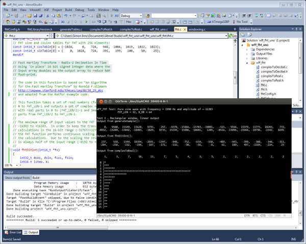
Screenshot of the FHT library output
The FHT Library
Overview
The FHT library is designed to compile on both AVR GCC and regular Linux GCC. As the library is completely written in C it should be very easy to port to other architectures and microcontroller types. The disadvantage of C is that it is not as efficient as coding the library in assembly language; however the desire (of the author) was to provide pedagogic code which could easily be sped-up by substituting core C functions with assembly equivalents. Having said this, the library is easily fast enough to provide real-time Fourier analysis even on a 16Mhz ATmega328P and requires around 17 ms to both permute the input and perform the FHT (of 256 inputs). Performance can be significantly improved by clocking the ATmega at its full 20Mhz if required.
By targeting both Linux and the ATmega328P the library could be more easily tested for overflow issues and portability issues (the library has also been tested on the ATmega32U4 which is found on the Arduino Leonardo board). It should be noted that some previous version of GCC had bugs in the 32-bit multiplication routines; so ensure that your compiler is up-to-date. When compiling with Atmel studio you must use at least version 6.1 to avoid the previously mentioned compiler bugs.
The library is configured using the fht/fhtConfig.h header file. The header file contains the various configuration options and explanations of what they do. The library also includes debugging functions which stream information about the FHT and associated functions to stdout. This allows the library to be tested on an Arduino Uno board using the serial output to monitor the results.
In addition to the library itself the Atmel Studio project and source code included with this article also provides an automatic testing tool for the FHT library which shows the generated input sample, the FHT output and the result of applying various window and scaling functions to the data.
The test results for the library are given in the following PDF files which show the output for FHT of lengths 32, 64, 128 and 256. Some rounding errors can be seen in the 256 length tests however these are mainly due to the way in which the input data is generated; with real audio data the library should function amicably even for lengths of 256.
FHT_Library_1_2_32_test_results
FHT_Library_1_2_64_test_results
FHT_Library_1_2_128_test_results
FHT_Library_1_2_256_test_results
Sampling
The FHT requires a sample of audio for processing. It is important that the samples are accurately spaced (i.e. have a consistent sampling rate) and the number of samples must match the input length of the FHT. The ADC function samples the audio intensity which can be considered as the average audio intensity over the duration of the sample. The result is a set of values which represent the intensity of the audio over the duration of the sampling.
The ATmega32U4 has a 10-bit ADC. This means that the range of results from the ADC is 0-1024. Since the audio input is AC this means our sample is in the range of -511 to +512 centred around 0.
The FHT function uses 16-bit integers however the FHT algorithm requires that the inputs are added and subtracted from each other. In order to do this in a 16-bit space the input to the FHT cannot exceed half the range of a 16-bit number i.e. -16384 to -16383. This limits the FHT resolution to 15 bits. Note that the FHT also requires multiplication of inputs, however this is performed using 32 bit temporary variables to preserve resolution and minimise RAM usage.
This means that, in order to get the maximum possible resolution from the FHT the 10 bit input samples need to be scaled up to 15 bits before being passed to the FHT.
The frequency range which can be supported by the FHT is based on the sampling rate of the input data. The highest frequency possible is limited by the Nyquist limit which states that the highest frequency which can be sampled is exactly half of the sampling rate. In other words, if you sample the audio at 20Ksps (20,000 samples per second) the maximum frequency you can detect is 10KHz. Any frequencies present in the input sample over the Nyquist limit will result in erroneous output by the FHT. Therefore care must be taken (in the hardware) to limit any frequencies over the Nyquist in the input signal to the ADC.
The library code includes a function generateSample() which simulates the sampling of audio data for testing purposes. When given an amplitude and frequency it passes back a sample of a pure sine-wave.
Windowing
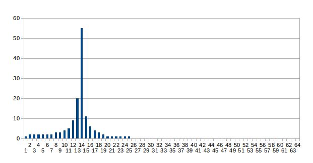
When sampling audio data using an ADC the samples are already windowed as sampling applies a rectangular window to the input audio. The issue with this is that, since the edges of the window are rectangular, the window can cause unwanted leakage of spectral components in the output of the FHT. This means that frequency components of the audio which get split between samples can result in errors from the FHT as the frequency components get spread out. The following diagram shows a 20Ksps sample of a 1500 Hz sine-wave without windowing:
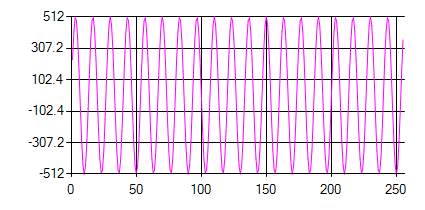
1500Hz Sine-wave at 20Ksps with no window function
To reduce this effect we can apply windowing functions to the input audio data. Windowing functions typically roll off the edges of the samples in order to reduce the spectral leakage (actually the spread the error across the sample to lessen its effect).
The FHT library supports 2 windowing functions (well, 3 if you include the default rectangular window), namely the Hann window and the Hamming window. These are popular windowing shapes for audio processing. The advantages and disadvantages of either are well documented on the web if you are interested in learning more about windowing functions.
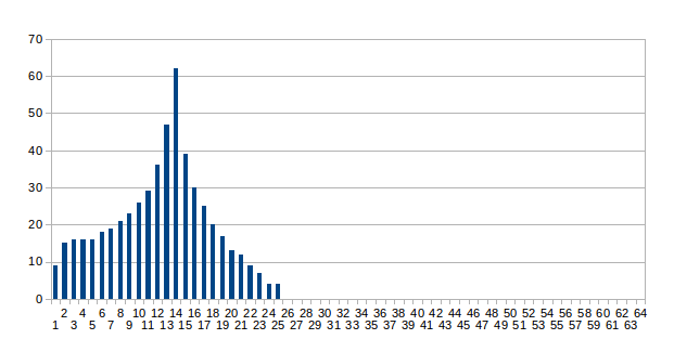
The same input sample shown above looks like the following diagram after having a Hamming window function applied to it:
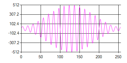
1500Hz Sine-wave at 20Ksps with Hamming window function
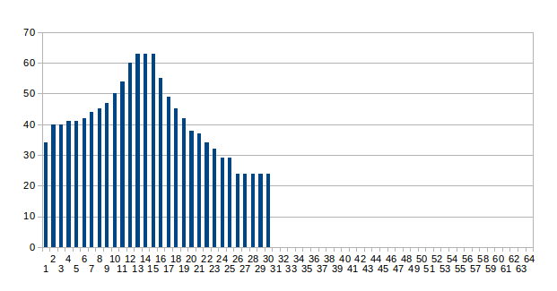
The diagram below shows the same sine-wave input, this time with a Hann window applied:
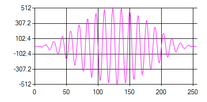
1500Hz Sine-wave at 20Ksps with Hann window function
It is worth noting that windowing functions come at a cost; whilst they improve the overall accuracy of the FHT output they also attenuate the input signal (i.e. remove some gain) which causes an overall drop in the resolution of the FHT.
To apply a Hann window to the sampled data you simply call applyHannWindow() and for a Hamming window you call applyHammingWindow().
The window function is applied using a look-up table to which the original sample is multiplied. The look-up tables are only half of the full window function (in order to save space) since both the Hann and Hamming window functions are symmetrical.
Fast Hartley Transformation
The FHT function accepts an input sample with a maximum of 256 components and each component must be in the range of -16384 to +16383. Any inputs outside of the accepted range will cause overflows in the FHT function and therefore unpredictable output. Care should be taken to scale the input data up to the maximum input range when possible as this ensures you get the maximum resolution from the FHT with minimum rounding errors.
The FHT is a decimation in time (DIT) transformation which takes the time-based intensities of the input sample and converts them to a frequency based representation. The output from the FHT is a set of complex numbers which represent the intensity of various frequencies ranges from the input sample.
The output from the FHT is a set of complex numbers with both real and imaginary parts. The first half of the output contains the real components of the output and the second half contains the imaginary components. This means that the output from FHT is exactly half the number of inputs (i.e. for a 256 component input you get 128 outputs).
To interpret the output from the FHT it is important to consider the sample rate of the processed audio. The FHT function operates on 32, 64, 128 and 256 sample inputs. The higher the number of inputs the more granular (narrow) the frequency ranges are. The output from the FHT is a series of frequency ‘bins’, the value of each bin represents the intensity of the input signal within the range of frequencies the bin represents. The exceptions to this are the first and last bins; the first bin is half as wide as the others (since it starts from 0 Hz) and the last bin contains the intensity at the Nyquist frequency (usually the first and last bins are ignored for most purposes). To demonstrate this (since it is at least a little confusing!) let’s consider an FHT with 32 input samples which were sampled at a rate of 20Ksps (thousand samples per second). The output bins represent an even spread of the frequencies from 0Hz to the Nyquist (in this case 10KHz) therefore the output bins have the following centre frequencies:
- 0: 0 Hz
- 1: 625 Hz
- 2: 1250 Hz
- 3: 1875 Hz
- 4: 2500 Hz
- 5: 3125 Hz
- 6: 3750Hz
- 7: 4375 Hz
- 8: 5000 Hz
- 9: 5625 Hz
- 10: 6250 Hz
- 11: 6875 Hz
- 12: 7500 Hz
- 13: 8125 Hz
- 14: 8750 Hz
- 15: 9375 Hz
Note that in the table above the first and last bins are narrower than the others. What this means is, for 32 input samples into the FHT, you get 14 usable frequency bins ranging from 312.5Hz to 9062.5Hz.
From an implementation standpoint it’s important to consider that the intensity of the input to the FHT is distributed across all bins in the output. Unless you are dealing with pure sine-waves of a single frequency the result of this is that, as you increase the number of inputs to the FHT, the average output intensity per bin drops. If you consider a complex input signal with equal intensities across all frequencies from 0Hz to the Nyquist (for the sake of example we will state that all frequencies have a input intensity of the maximum allowed by the FHT function i.e. +16384) then the output for a 32 bin FHT will be 16384/32 = 512, however for a 64 bin FHT the average will be 16384/64 = 128. This is an issue when interpreting the output since higher number of bins will result in smaller average outputs; since the input resolution from the ADCs is fixed you get less and less resolution in the output as you increase the number of bins.
Usually this effect is avoided by showing a smaller range of output at less resolution and clipping any results over a certain intensity (which is what the complexToDecibelWithGain() function does – see below). This is ok if you are just after a visual representation of the audio, but not suitable for audio analysis applications where the actual intensity is required. Even though the FHT function can support more than 256 FHT inputs the resolution becomes so little in the output that it is not really useful unless you can increase the resolution of the input to compensate.
In order to keep the FHT calculations in the range of a 16 bit integer the FHT function continuously scales the output of the calculations (by dividing them in half). The net result of this is that the output is exactly half the value of the input (i.e. if you put 16834 in you get 8192 out).
The FHT is called using the fhtDitInt() function. Care must be taken to ensure that the FHT_LEN and FHT_SCALE parameters are set at compilation time to ensure the length of the FHT input data is correct.
For audio sample analysis the output of the FHT is not useful unless it is converted into a linear or logarithmic representation of amplitude. You will need to run either the linear or decibel conversion functions (see below) on the FHT output to get meaningful results.
Complex to real number conversion (linear)
Since the output from the FHT is in the form of complex numbers you need to convert the complex numbers into real numbers before displaying the output from the FHT. To do this you need to take the power of 2 of both the real and imaginary parts, add them together and take the square-root of the result (this is the absolute of the complex number):
fx(k) = SQRT( (fx(k)^2) + (fx(-k)^2) )
This formula gives the linear intensity of the FHT output bin and has to be applied to all output bins.
The library function complexToReal() performs the formula above on the input data and also provides the ability to scale the output. By default (with a scale of 0) the function will output scaled results in the range 0-8192. This output can be further scaled by providing a positive scaling factor to the function. For example, a scale of 7 causes the output data to be scaled by 2^7 = 128 giving results in the range of 0-63. This scaling is very useful if your output device is a display since you can easily scale the output to the resolution of the display using this function.
The following chart shows the output from a 1990Hz sine-wave sampled at 20Ksps through a 128 point FHT with rectangular windowing. The result is linear and has been scaled to a range of 0-63:
1990Hz Sine-wave at 20Ksps linear output
Complex to decibel conversion (logarithmic)
When analysing frequencies the linear intensity is useful but does not give a representation which mirrors how we hear sounds. In reality if you want to double the ‘loudness’ of a sound you must double the linear intensity at each step, for example, if you double the loudness of a sound with an intensity of 512 the intensity becomes 1024, if you want to double it again it becomes 2048. This logarithmic representation of the sound intensity is typically given in decibels.
To get from a linear intensity to a decibel representation you need to first convert the complex number into a absolute number and then scale it into decibels according to the following formula:
linear intensity = sqrt(re * re + im * im)
dB = 20 * log10(linear intensity)
Since decibel is a relative measurement we have to consider the ADC input when converting. The two important factors are the maximum input value (refV which is 5V or +16383 units into the FHT) which represents the maximum intensity (and therefore 0dBs) and the actual input value which is in the range of 0 to refV. So, in reality our input signal in dBs is represented by the following formula:
dBV = 20 * log10(V / refV)
To produce a decibel look up table we need to take into account the smallest amount of input we can measure (since the decibel scale is from 0 dBs to infinity). This is the ‘noise floor’ of the signal (i.e. below this level the real signal is indistinguishable from the noise level).
The complexToDecimal() function uses a look up table with values representing steps of linear intensity which represent decibel amounts. If you reverse the formula above to represent it in terms of the linear intensity you get:
V = refV * 10^(dBV / 20)
This is the formula that is used to generate the required linear to decibel look up table. The function simply steps through the table to find the required intensity and then takes the array index as the decibel equivalent. If the scale is -75 dB to 0 dB and the array is 64 values then each index of the array represents -1.172 dBs (-75 / 64). It should be noted that the result is relative to the actual input intensity i.e. what 0 dBs really represents is whatever the input signal is at maximum intensity.
The size of the look-up table provides the overall scale of the result. With N_DB set to 64 the output is 0-63, alternatively you can set N_DB to 128 for an output of 0-128. If you require other ranges you must regenerate the required look-up tables using the provided table generation functions.
The following chart shows the output from a 1990Hz sine-wave sampled at 20Ksps through a 128 point FHT with rectangular windowing. The result is logarithmic and has been scaled to a range of 0-63 where 0 dB is 63 and -78 dB is 0:
1990Hz Sine-wave at 20Ksps logarithmic decibel output
Complex to decibel conversion with gain
The complex to decibel conversion with gain function is similar to the previous function however the table is modified to scale the output differently. By raising the noise floor value or lowering the maximum intensity in the look up table you can increase the gain on smaller intensities at the expense of clipping intensities which are over the maximum. This allows you to use the function to ‘zoom in’ on a part of the output. Although this is not really useful for audio analysis it is useful when displaying the FHT output as a representation of the input sound sample as it provides more detail about smaller intensities when displaying the results. In order to be useful the table needs to be tweaked based on the expected intensity of the input and the average intensity of the FHT output which is very application specific.
The following chart shows the output from a 1990Hz sine-wave sampled at 20Ksps through a 128 point FHT with rectangular windowing. The result is logarithmic and has been scaled to a range of 0-63 where -30 dB is 63 and -78 dB is 0:
1990Hz Sine-wave at 20Ksps logarithmic decibel output with gain
Compiling the library
The zip file provided below contains all the required source code for the library in a Atmel Studio 6.1 project. To run the library without alteration use Atmel Studio to program the code (via ICSP) to an Arduino Uno development board. The only architecture dependent code is the USART routines which provide debug output via the Uno’s USB to serial converter. If you wish to run the code on another board then start by altering the usart.c library to your target chip.
You can also use the source-code as the basis for an Eclipse project under Linux. You can set the configuration of the fhtConfig.h header to target either AVR or Linux; the library will automatically change the required include files and use either stdio.h or the usart code for printf output. The library will also only attempt to put the pre-calculated tables in PROGMEM when targeting AVR environments, otherwise the tables are loaded into RAM.
Make sure you use either Atmel Studio 6.1 or an up-to-date version of GCC as older versions contain 32 bit multiplication bugs which can prevent the library from functioning correctly.
Generating the pre-calculated tables
The library contains a function called generateTables() which calculates the data for all of the tables used in the library. The output is ready formatted as C code so you can simply cut and paste the output back in to the source files. The generateTables.c file includes lots of comments about how the table generation works which should give you the information you need if you want to alter the tables for your own purposes.
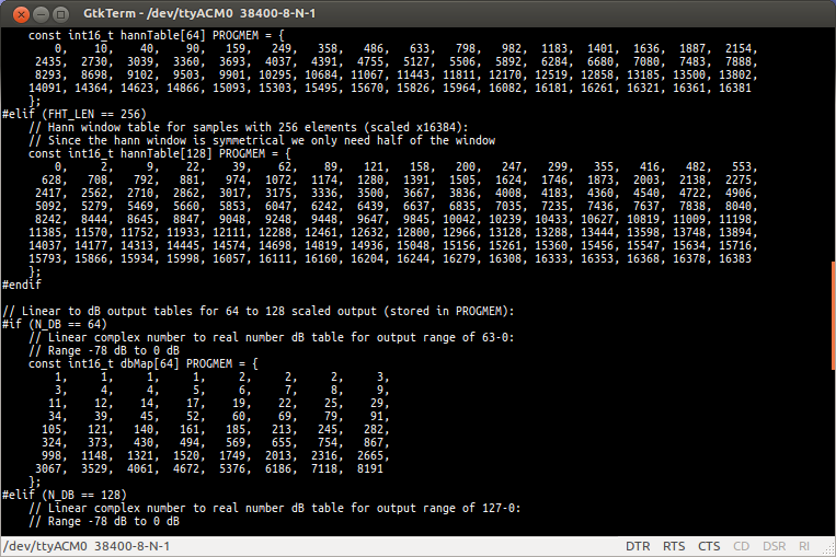
Automatic table generation output
References and citations
The FHT function in the library is based on “An Algorithm for the Fast Hartley Transform” by Ronald F.Ullmann and adapted from the Ratfor example code. The original article can be downloaded (as a PDF) from the following link:
[http://sepwww.stanford.edu/theses/sep38/38_29_abs An Algorithm for the Fast Hartley Transform]
An Algorithm for the Fast Hartley Transform
I’d like to thank the kind help and advice given over at Open Music Labs Forums and for their AVR assembly FHT library for the Arduino which was a great help when developing my own library:
Files for download
This zip file contains the AVR Studio 6.1 firmware project files for the FHT library and the test code:
Hello, since there’s no forum anymore, i will ask a question here. First of all, i want again to thank you for all you do! As I understood, number of output bands are connected to FHT_LEN number as FHT_LEN/2? Is there’s possibility to get for example 8 frequency ranges? I had idea to get like FHT_LEN = 64, after that i will get 32 ranges, and then sum first, second, third and fourth result and so on for every 4 ranges.
You can either change the overall number of frequency buckets (by changing the length of the FHT) or you can take an average of the buckets to get the range you want.
Both ways have advantages: Dropping the number of buckets overall speeds up the FHT calculations. Taking the averages gives you the ranges without loosing resolution for other tasks.
It’s up to you which you choose depending on your overall purpose.
So I can change FHT_LEN to 16 so i will get 8 buckets?
Yes, should be just a case of modifying fht/fhtConfig.h; just be aware that your sample rate will be the thing controlling what frequencies the buckets actually contain.
Yeah, it works. But height of bar decrease as frequency goes up.
Ah no, its something wrong with getting samples, because all fine when i tryed generateSameples function.
Also, Simon, is it possible to make forum once again? I think its much more useful than this commenting system, because allows to post pictures, edit, easily navigate among different topics etc.
Unfortunately not; the forum just generated too much overhead – also it was too specialised – there are a large number of electronics forums already on the web where you can seek general electronics help.
Hi Simon,
I tried to execute the FHT of a sin and cos at same frequency, but I got the same result. In the FFT theory the output for sin is imaginary, while the output of cos is real.
Why did i get to real result?
The FHT/FFT expects periodic signals. Are you inputting a number of waves or a single wave? Also rounding errors in the calculation can lead to false-positives in the frequency outputs.
Two simulations with:
signal frequency 50Hz
Samples per second 1600 (4 periods)
number of input samples: 128
Amplitude: 100
1) double floatCalc = (amplitude * cos (radiansPerSecond * time));
2) double floatCalc = (amplitude * sin (radiansPerSecond * time));
But in the 4th harmonic I always get a real result.
Attached the output of cos and sin
https://wetransfer.com/downloads/b3a849d8e39dc5275ff9ebef713ae1cb20171002103936/0a43c3f145c5d80f21279c9dd26187ad20171002103936/cc36bc
Thanks